Sparse approximation

Sparse approximation (also referred to as sparse decomposition) is the problem of estimating a sparse multi-dimensional vector, satisfying a linear system of equations given high-dimensional observed data and a design matrix. Sparse approximation techniques have found wide use in applications such as image processing, audio processing, biology, and document analysis.

1 Sparse decomposition
- 1.1 Noiseless observations
- 1.2 Noisy observations
2 Variations
- 2.1 Structured sparsity
- 2.2 Collaborative sparse coding
3 Algorithms
4 References

Sparse decomposition

Noiseless observations

Consider a linear system of equations $x = D\alpha$ , where $D$ is an $m\times p$ matrix $(m \ll p)$ and $x \in \mathbb{R}^m,\alpha \in \mathbb{R}^p$ . $D$ , called as the dictionary or the design matrix, is given. The problem is to estimate the signal $\alpha$ , subject to the constraint that it is sparse. The underlying motivation for sparse decomposition problems is that even though the observed values are in high-dimensional $(m)$ space, the actual signal is organized in some lower-dimensional subspace $(k \ll m)$ .

Sparsity implies that only a few components of $x$ are non-zero and the rest are zero. This implies that $x$ can be decomposed as a linear combination of only a few $m\times 1$ vectors in $D$ , called atoms. $D$ itself is over-complete $(m \ll p).$ Such vectors are called as the basis of $x$ . However, unlike other dimensionality reducing decomposition techniques such as Principal Component Analysis, the basis vectors are not required to be orthogonal.

The sparse decomposition problem is represented as,

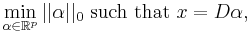
$\min_{\alpha \in \mathbb{R}^p} ||\alpha||_0 \text{ such that } x = D\alpha,$

where $||\alpha||_0 = \#\{ i�: \alpha_i \neq 0, \, i=1,\ldots,p \}$ is a pseudo-norm, $l_0$ , which counts the number of non-zero components of $\alpha = [\alpha_1,\ldots,\alpha_p]^T$ . This problem is NP-Hard with a reduction to NP-complete subset selection problems in combinatorial optimization. A convex relaxation of the problem can instead be obtained by taking the $l_1$ norm instead of the $l_0$ norm, where $||\alpha||_1 = \sum_{i=1}^p |\alpha_i|$ . 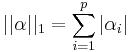The $l_1$ norm induces sparsity under certain conditions^[1].

Noisy observations

Often the observations $x$ are noisy. By imposing an $l_2$ norm on the data-fitting term and relaxing the equality constraint, the sparse decomposition problem is given by,

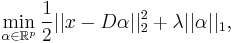
$\min_{\alpha \in \mathbb{R}^p} \frac{1}{2} ||x - D\alpha ||_2^2 %2B \lambda ||\alpha||_1,$

where $\lambda$ is a slack variable and $||\alpha||_1$ is the sparsity-inducing term. The slack variable balances the trade-off between fitting the data perfectly, and employing a sparse solution.

Variations

There are several variations to the basic sparse approximation problem.

Structured sparsity

In the original version of the problem, any atoms in the dictionary can be picked. In the structured (block) sparsity model, instead of picking atoms individually, groups of atoms are to be picked. These groups can be overlapping and of varying size. The objective is to represent $x$ such that it is sparse in the number of groups selected. Such groups appear naturally in many problems. For example, in object classification problems the atoms can represent images, and groups can represent category of objects.

Collaborative sparse coding

The original version of the problem is defined for only a single point $x$ and its noisy observation. Often, a single point can have more than one sparse representation with similar data fitting errors. In the collaborative sparse coding model, more than one observation of the same point is available. Hence, the data fitting error is defined as the sum of the $l_2$ norm for all points.

Algorithms

There are several algorithms that have been developed for solving sparse approximation problem.

Matching pursuit

Matching Pursuit is a greedy iterative algorithm for approximatively solving the original $l_0$ pseudo-norm problem. Matching pursuit works by finding a basis vector in $D$ that maximizes the correlation with the residual (initialized to $x$ ), and then recomputing the residual and coefficients by projecting the residual on all atoms in the dictionary using existing coefficients. Matching pursuit suffers from the drawback that an atom can be picked multiple times which is addressed in orthogonal matching pursuit.

Orthogonal matching pursuit

Orthogonal Matching Pursuit is similar to Matching Pursuit, except that an atom once picked, cannot be picked again. The algorithm maintains an active set of atoms already picked, and adds a new atom at each iteration. The residual is projected on to a linear combination of all atoms in the active set, so that an orthogonal updated residual is obtained. Both Matching Pursuit and Orthogonal Matching Pursuit use the $l_0$ norm.

LASSO

LASSO method solves the $l_1$ norm version of the problem. In LASSO, instead of projecting the residual on some atom as in Matching Pursuit, the residual is moved by a small step in the direction of the atom iteratively.

Other methods

There are several other methods for solving sparse decomposition problems ^[2]

Homotopy method
Coordinate descent
First order/proximal methods
Dantzig selector^[3]

References

^ Donoho, D.L. (2006). "For most large underdetermined systems of linear equations the minimal l1-norm solution is also the sparsest solution". Communications on pure and applied mathematics (Wiley Online Library) 56 (6): 797–829.
^ Francis Bach, Julien Mairal, Jean Ponce and Guillermo Sapiro. "Sparse Coding and Dictionary Learning for Image Analysis". http://www.di.ens.fr/~mairal/tutorial_iccv09/tuto_part1.pdf.
^ Candes, Emmanuel; Tao, Terence (2007). "The Dantzig selector: Statistical estimation when p is much larger than n". Annals of Statistics 35 (6): 2313–2351. arXiv:math/0506081. doi:10.1214/009053606000001523. MR 2382644.

Numerical linear algebra

Key concepts	Floating point · Numerical stability · BLAS

Problems	Matrix multiplication · Matrix decompositions · Linear equations · Sparse problems

Hardware	CPU cache · TLB · Cache-oblivious algorithm · SIMD · Multiprocessing

Software	Specialized libraries · General purpose software